 |
 |
| • | BallHill: | Ball rolling on a height field subject to gravitational force. |
| • | BallRubberBand: | Ball attached to point with rubber band; Lagrangian dynamics. |
| • | BeadSlide: | Bead sliding on frictionless wire; Lagrangian dynamics. (GP, Exercise 3.7). |
| • | BlownGlass: | A 3D fluid simulation is used to generate a dynamic volumetric texture on a surface. |
| • | BouncingBall: | Deformation; implicit surface extraction to generate ball. |
| • | BouncingSpheres: | Collision detection and response of spheres using impulse-based methods. |
| • | BouncingTetrahedra: | Collision detection and response of tetrahedra using impulse-based methods. |
| • | Cloth: | Illustration of a 2-dimensional mass-spring system (CPU). |
| • | CollisionsBoundTree: | Collision detection using a bounding-volume hierarchy. |
| • | CollisionsMovingSpheres: | Collision detection for two moving spheres. |
| • | CollisionsMovingSphereTriangle: | Collision detection for a moving sphere and a moving triangle. |
| • | DoublePendulum: | Two rods, two joints with one fixed, no friction; Lagrangian dynamics. |
| • | FlowingSkirt: | Deformation of generalized cylinder surfaces. |
| • | Fluids2D: | A GPU-based 2D fluid simulation using the Navier-Stokes equations. |
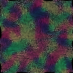
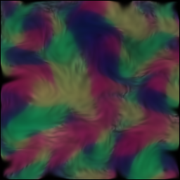
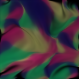
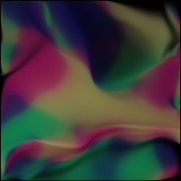
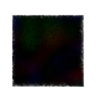
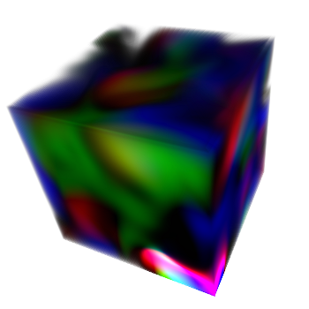
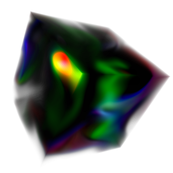
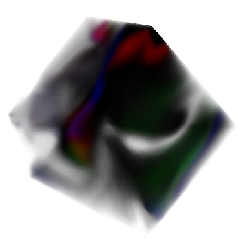
| • | Fluids3D: | A GPU-based 3D fluid simulation using the Navier-Stokes equations. |
| • | FoucaultPendulum: | Solving the equations of motion for the Foucault Pendulum. |
| • | FreeFormDeformation: | Deformation; free-form with B-spline volumes. |
| • | FreeTopFixedTip: | A spinning top whose tip is attached to ground; Euler's equations. |
| • | GelatinBlob: | Mass-spring system, arbitrary topology (icosahedron). |
| • | GelatinCube: | Mass-spring system, 3D array topology. |
| • | HelixTubeSurface: | Tube surfaces. |
| • | IntersectingBoxes: | All-pairs box intersections using sort-and-sweep. (GP, Page 360.) |
| • | IntersectingRectangles: | All-pairs rectangle intersections using sort-and-sweep. (GP, Page 359.) |
| • | KeplerPolarForm: | Solving equations of motion for Earth-Sun. |
| • | MassPulleySpringSystem: | Complex system; Lagrangian dynamics. |
| • | MassSprings3D: | A GPU-based 3D mass-spring system solved using a Runge-Kutta 4th-order method (32768 masses). |
| • | Rope: | Illustration of a 1-dimensional mass-spring system (CPU). |
| • | RoughPlaneFlatBoard: | Flat board moving on a plane with friction. |
| • | RoughPlaneParticle1: | Particle moving on a plane with friction. |
| • | RoughPlaneParticle2: | Two particles attached by massless rod moving on a plane. |
| • | RoughPlaneSolidBox: | Solid box moving on a plane with friction. |
| • | RoughPlaneThinRod1: | Thin rod moving on a plane with friction (full physics, slow). |
| • | RoughPlaneThinRod2: | Thin rod moving on a plane with friction (approximate physics, fast). |
| • | SimplePendulum: | Solving equations of motion for a pendulum with frictionless joint. |
| • | SimplePendulumFriction: | Solving equations of motion for a pendulum, friction at joint. |
| • | WaterDropFormation: | Deformation of revolution surfaces to simulate water-drop formation. |
| • | WrigglingSnake: | Deformation of tube surfaces to simulate motion of a snake. |
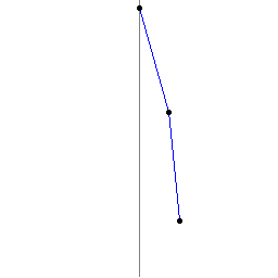
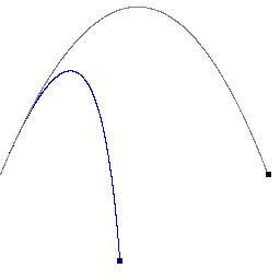
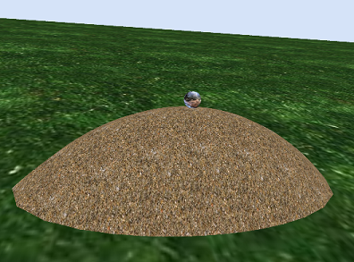
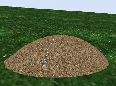
BallHill. Ball rolling on a height field subject to gravitational force.
A ball is placed at the top of a hill whose shape is an elliptical paraboloid. The hill
is assumed to be frictionless. The only force acting on the ball is gravitational force.
The ball is slightly pushed so that it may slide down the hill. The second image shows
the path of the center of the ball as it rolls down the hill. The ball rotates at a
speed commensurate with its downhill velocity.
|
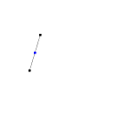
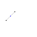
BallRubberBand. Ball attached to point with rubber band; Lagrangian dynamics
A ball is attached by an elastic string to a fixed point on a table. The ball is given
an initial velocity whose direction is not towards the fixed point. The path must be
an ellipse. The ball's path starts in green, finishes in blue, and is a blend of the
two colors between.
|
| BeadSlide. Bead sliding on frictionless wire; Lagrangian dynamics. (GP, Exercise 3.7) A bead is placed at a location on a spiral curve. The bead is subject only to gravitational force. This program computes the position of the bead for various times. The application is a console one. For an exercise, write a 3D graphics program to display the moving bead. |
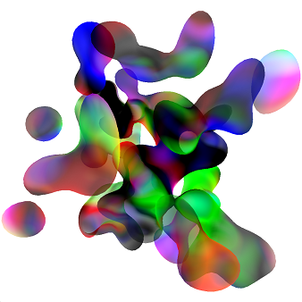
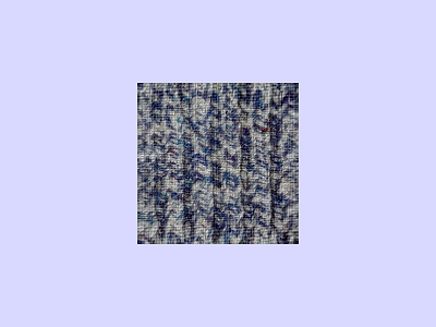
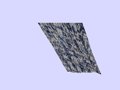
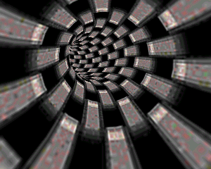
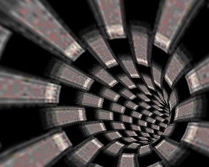
BlownGlass. The example is a mixture of
graphics, surface extraction and fluid dynamics. The vertex and index
data were generated by the Sample/Imagics/SurfaceExtraction sample. The
surfaces are embedded in a dynamic 3D texture that is generated by the
Sample/Physics/Fluids3D. This sample was used to generate the book cover
art for GPGPU Programming for Games and Science.
A 3D fluid simulation on a lattice generates a dynamic 3D texture that
is applied to a 2D surface embedded in the lattice. The left image is
a screen capture obtained during the simulation. The right image is the
GPGPU Programming for Games and Science book cover.
|
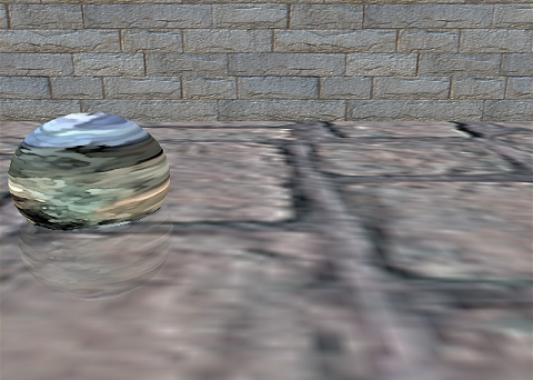
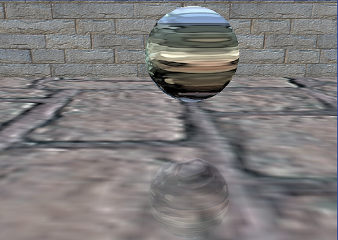
BouncingBall. Deformation; implicit surface extraction to generate ball.
A deformable body initially in the shape of a sphere is bounced on a floor.
When the body hits the floor, it starts to deform. At the instant of maximum
deformation, the body bounces off the floor and gradually returns to its spherical
shape. The reflection of the ball on the floor allows you to see some of the
deformation occurring. The application allows you to supply an alternate
deformation via nonuniform scaling.
|
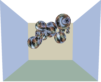
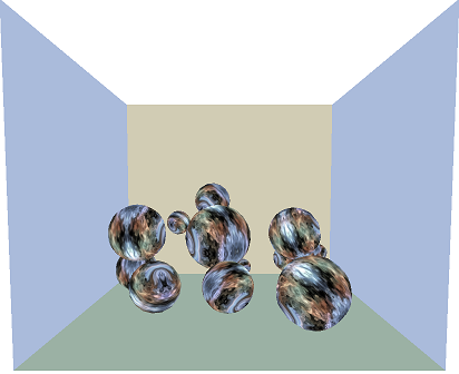
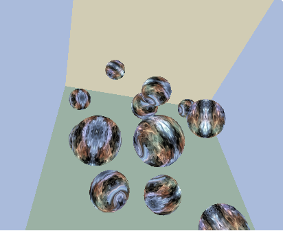
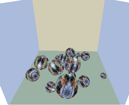
BouncingSpheres. Collision detection and response of spheres using impulse-based methods.
A collection of spheres of various radii are bouncing around in a room. The
front wall and ceiling are not rendered so that you can rotate the virtual
trackball to see the simulation from various perspectives. The physics is
based on impulsive forces (acceleration-based methods). The upper-left image
is the initial configuration of the simulation. The upper-right image occurs
at simulation time 2.658. The lower-left image shows the same simulation time
but with the scene rotated by the virtual trackball. The lower-right image shows
the final steady-state configuration of the simulation; the balls have stopped
moving.
|
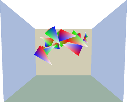
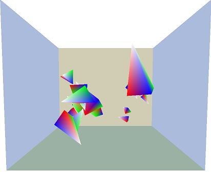
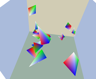
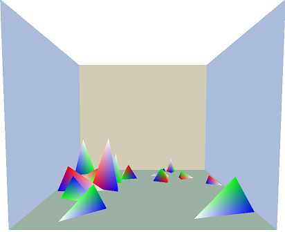
BouncingTetrahedra. Collision detection and response of tetrahedra using impulse-based methods.
A collection of tetrahedra of various sizes are bouncing around in a room. The
front wall and ceiling are not rendered so that you can rotate the virtual
trackball to see the simulation from various perspectives. The physics is
based on impulsive forces (acceleration-based methods). The upper-left image
is the initial configuration of the simulation. The upper-right image occurs
at simulation time 1.683. The lower-left image shows the same simulation time
but with the scene rotated by the virtual trackball. The lower-right image shows
the final steady-state configuration of the simulation; the tetrahedra have stopped
moving.
|
Cloth. Illustration of a 2-dimensional mass-spring system.
A cloth is modeled as a rectangular array of springs. Wind forces make
the cloth flap about. Notice that the cloth in the bottom image is
stretched in the vertical direction. The stretching occurs while the
gravitational and spring forces balance out in the vertical direction
during the initial portion of the simulation.
|
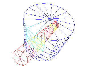
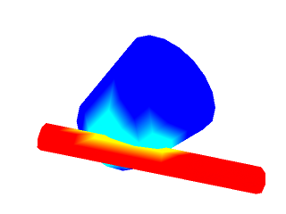
CollisionsBoundTree. Collision detection using a bounding-volume hierarchy.
The application demonstrates the simple use of oriented bounding box trees
for collision detection between two cylinders. One cylinder is drawn in blue,
the other in red. Whenever a pair of triangles intersects, one from each
cylinder, the blue-cylinder triangle's vertex colors are changed to cyan and
the red-cylinder triangle's vertex colors are changed to yellow. The initial
configuration of cylinders is shown in the next images. The blue cylinder is
intersected on its top and bottom disks. The red cylinder is intersected on
its wall.
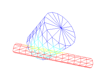
The scene may be rotated using left-mouse drags on a virtual trackball. The red cylinder may be rotated using the keys 'r'/'R', 'y'/'Y', and 'p'/'P'. The next two images show the results of rotating the red cylinder. Notice that the red cylinder does not intersect the blue cylinder on its top disk, yet some of the top-disk triangles have a tint of cyan. This is due only to coloring the vertices of those blue-cylinder triangles that are intersected by the red cylinder. There is a sharp cutoff of cyan/blue on the right-most intersected triangles of the blue cylinder. This is due to the cylinder being built from a rectangle mesh that is wrapped around whereby the vertices at the cylinder seam are duplicated.
The red cylinder may be translated using the keys 'x'/'X', 'y'/'Y', and 'z'/'Z'. The next two images show the results of translating the red cylinder.
|
CollisionsMovingSpheres. Collision detection for moving spheres.
The application implements the pseudocode of Sections 8.3.1 and 8.3.2
of 3D Game Engine Design, 2nd edition.
Two spheres are moving with constant linear velocities. They are constrained
to lie inside a larger bounding sphere (invisible in the application), so as
each sphere hits the bounding sphere, it is reflected accordingly with no
loss of energy. When the two moving spheres collide, they are each reflected
accordingly with no loss of energy. This is a continuous collision detection
algorithm whereby the collisions are predicted continuously in time, not by
taking discrete time steps and bisecting to find the contact time. The three
screen captures show the spheres before contact (left), the spheres at
contact (middle), and the spheres after contact (right). The arrows
were hand drawn into the screen captures to show the directions of motion.
|
|
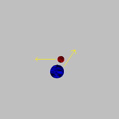
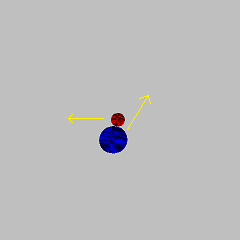
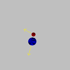
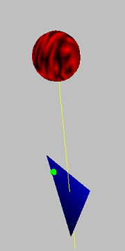
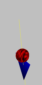
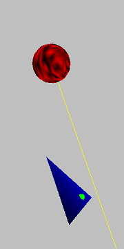
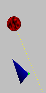
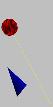
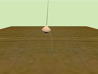
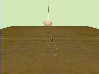
CollisionsMovingSphereTriangle. Collision detection for a moving sphere
and a moving triangle. The algorithm is equivalent to a ray-tracing algorithm.
The PDF describes an equivalent Voronoi-based approach that should be more
efficient computationally than the ray-tracing algorithm.
The application shows a sphere and a triangle. The triangle is stationary and
the sphere is "moving" in the sense that it is assigned a constant linear
velocity and the application predicts the contact point with the triangle.
The yellow line shows the path of the moving sphere center. The green sphere
shows the predicted contact point. The scene is controlled by a virtual track
ball. You can select the red sphere to be controlled by the track ball.
Rotation of the sphere is converted to a rotation of the velocity vector (you
see the yellow line move). You can also select the blue triangle to be controlled
by the track ball. If the sphere is predicted not to intersect the triangle, the
green sphere disappears.
The first image shows the sphere, triangle, path of center, and predicted contact point. You can press the space bar to move the sphere along the velocity direction for the computed contact time. At this time the sphere is in contact with the triangle (you cannot see the green sphere unless you toggle to wireframe mode). The second image shows the sphere in contact with the triangle. The third image shows the sphere after rotating it with the virtual track ball. The fourth image shows more rotation that leads to a contact point closer to the right-most triangle vertex. The fifth image shows yet more rotation that leads to the sphere missing the triangle, so the green sphere is gone (indicating no-intersection).
|
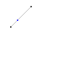
DoublePendulum. Two rods, two joints with one fixed, no friction; Lagrangian dynamics.
A double pendulum with two masses connected by rigid rods. The screen shots show
the system at two times during the simulation. The left image shows the initial
configuration. Both masses start with zero angular speed. The right image is at
a time soon after the initial time.
|
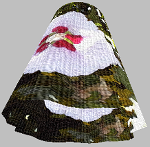
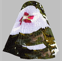
FlowingSkirt. Deformation of generalized cylinder surfaces.
A skirt modeled by a generalized cylinder surface. Wind-like forces are acting on the
skirt and are applied in the radial direction. The top image shows the skirt after
wind is blowing it about. The bottom image shows a wireframe view of the skirt so that
you can see it consists of two closed curve boundaries and is tessellated between.
|
Fluids2D. A GPU-based 2D fluid simulation. The bulk of the source code,
including HLSL shaders embedded as std::string objects, is in the
GTEngine project.
The screen captures are, from left-to-right then top-to-bottom, for
frames 0, 16, 32, 64, 256, and 512. The fluid is subject to various
forces (wind, gravity, vortices). The pseudocoloring is based on
velocity (mapped to r, g, b) and modulated by density. The initial
density is generated randomly using a uniform distribution.
|
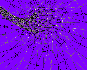
Fluids3D. A GPU-based 3D fluid simulation. The bulk of the source code,
including HLSL shaders embedded as std::string objects, is in the
GTEngine project.
The screen captures are, from left-to-right then top-to-bottom, for
various frames over time. The fluid is subject to various
forces (wind, gravity, vortices). The pseudocoloring is based on
velocity (mapped to r, g, b) and modulated by density. The initial
density is generated randomly using a uniform distribution. The
data is volume rendered using nested boxes for geometry. Alpha
blending is used, where the alpha channel is proportional to the density.
|
|
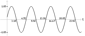
FoucaultPendulum. Solving equations of motion for Foucault pendulum. (GP, Example 3.3) The figures show the path of the pendulum tip in the horizontal plane. New points on the path are colored white but the intensity of the older points along the path gradually decreases.
|
|
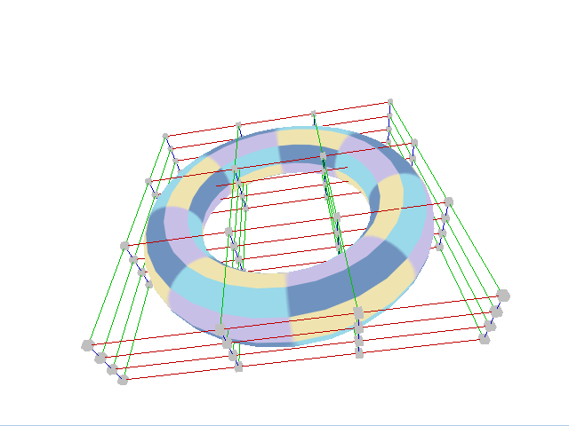
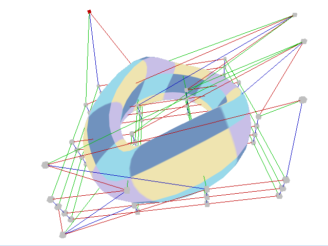
FreeFormDeformation. Deformation; free-form with B-spline volumes The left image shows the initial configuration where all control points are rectangularly aligned. The right image shows that some control points have been moved and the surface is deformed. The control point shown in red in the bottom image is the point at which the mouse was clicked on and moved.
|
|
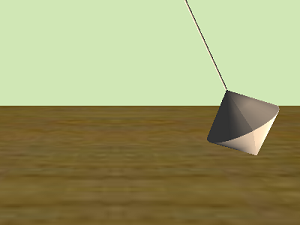
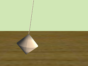
FreeTopFixedTip. A spinning top whose tip is attached to ground; Euler's equations. Two snapshots of a freely spinning top taken with two camera poses. The black line is the vertical axis. The white line is the axis of symmetry f the top. The top rotates about its axis of symmetry and the axis of symmetry rotates about the vertical axis.
|
|
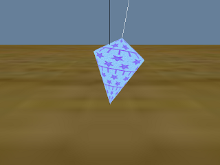
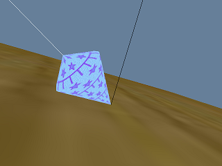
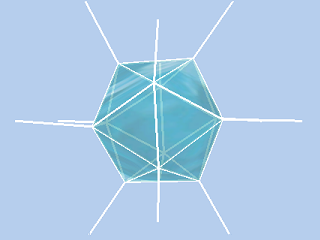
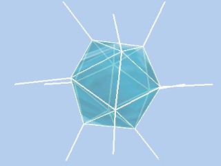
GelatinBlob. Mass-spring system, arbitrary topology (icosahedron). A gelatinous blob that is oscillating due to small, random forces. This blob has the masses located at the vertices of an icosahedron with additional masses of infinite weight to help stabilize the oscillations. The springs connecting the blob to the infinite masses are shown in white.
|
GelatinCube. Mass-spring system, 3D array topology.
A gelatinous cube that is oscillating due to random forces. The cube is
modeled by a three-dimensional array of mass connected by springs. To make
the visual appearance more realistic, the faces of the cube have some
transparency. As the cube is rotated, the drawing order of the faces is
updated to make sure the alpha blending is correct.
|
HelixTubeSurface. Tube surfaces.
A closed tube that is built as a double helix with constant radius. This is
the typical tube demonstration that folks like to build. You can modify this
application to use whatever closed curve you have in mind.
|
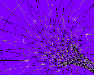
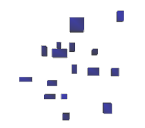
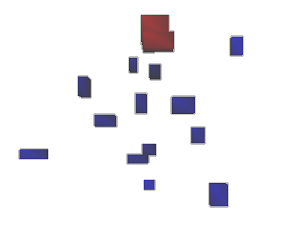
IntersectingBoxes. All-pairs box intersections using sort-and-sweep. (GP, Page 360.)
A collection of axis-aligned bounding boxes are randomly moving about in space. The boxes
are blue initially. Whenever two boxes intersect, their colors are changed to red. The
intersection testing uses time coherency to speed up the collision detection system.
|
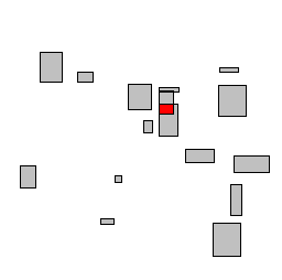
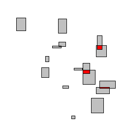
IntersectingRectangles. All-pairs rectangle intersections using sort-and-sweep. (GP, Page 359.)
A collection of axis-aligned rectangles are randomly moving about in the plane.
The boxes are gray initially. Whenever two rectangles intersect, their colors
are changed to red. The intersection testing uses time coherency to speed up
the collision detection system.
|
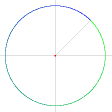
KeplerPolarForm. Solving equations of motion for Earth-Sun.
The red dot represents the Sun. The elliptical path is the orbit of the Earth around the Sun.
The sun is at a focal point of the ellipse, which is not at the center of the ellipse but is
close to the center. The orbit starts in green, finishes in blue, and is a blend of the two
colors between.
|
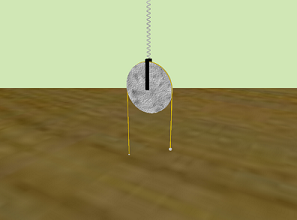
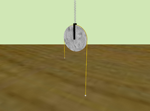
MassPulleySpringSystem. Complex system; Lagrangian dynamics.
A mass pulley spring system shown at two different times. The spring
expands and compresses and the pulley disk rotates during the simulation.
The system stops when a mass reaches the center line of the pulley or the
ground.
|
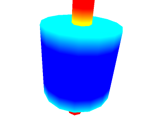
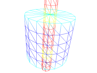
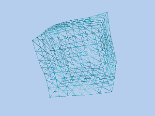
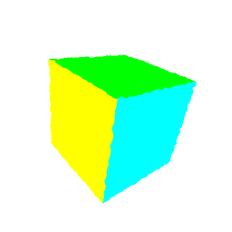
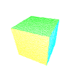
MassSprings3D. A GPU-based mass-spring system, where the particles are vertices in a 3D lattice
and the springs connect particles in the coordinate axis directions. The application
is not visually interesting, but shows that you can process a very large mass-spring
system in real time. The lattice has 323 (32768) masses. The GPU version
runs at 2300 frames per second on an AMD 7970. The CPU version is also provided to
show you how much faster the GPU version is; the CPU version runs at 80 frames per
second. Effectively, this shows how you can numerically solve systems of ordinary
differential equations on the GPU.
The left image is a solid view of the lattice of masses and the right image
is a wire-frame view. When simulating, the masses oscillate slightly so
that you can see the simulation is actually running.
|
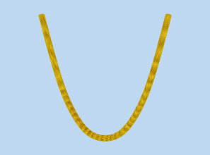
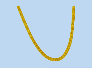
Rope. Illustration of a 1-dimensional mass-spring system.
A rope modeled as a linear chain of springs. The left image shows the
rope at rest with only gravity acting on it. The right image shows the
rope subject to a wind force whose direction changes by small random
amounts.
|
RoughPlaneFlatBoard. Flat board moving on a plane with friction.
A flat board in the shape of a rectangle moves on a horizontal planar surface. The
surface exerts a frictional force on the board. A physics hack is used to decouple
the equations for the center of mass and the angular velocity. This avoids an
expensive numerical integration that the generalized forces would require. The
images show a couple of snap shots of the board which was initially given a nonzero
linear and angular velocity. The center of mass moves from upper left to lower right.
The rectangle rotates counterclockwise about its center of mass.
|
RoughPlaneParticle1. Particle moving on a plane with friction.
A particle moves on a planar surface that is slanted relative to the xy-plane.
The particle is affected by gravitational force. The surface exerts a frictional
force on the particle. The screen shot shows the path of the particle, which was
given an upward initial velocity. The gray path corresponds to an application of
rough friction. In contrast, the blue path corresponds to an application of
viscous friction.
|
RoughPlaneParticle2. Two particles attached by massless rod moving on a plane.
Two particles consider to be a rigid particle system move on a horizontal planar
surface. The surface exerts a frictional force on the particles. The particle system
is initially given nonzero linear and angular velocities. Eventually the system stops
moving. The images show a couple of snap shots in time of the system. The center of
mass moves diagonally from upper left to lower right. The rod is rotating
counterclockwise about its center of mass.
|
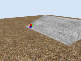
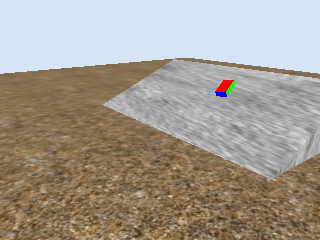
RoughPlaneSolidBox. Solid box moving on a plane with friction.
A solid box moves on a planar surface that is slanted relative to the xy-plane.
The box is affected by gravitational force. The surface exerts a frictional force
on the bottom of the box. A physics hack is used to decouple the equations for
the center of mass and the angular velocity. This avoids an expensive numerical
integration that the generalized forces would require. The images show the box at
various times in the simulation. The box is given an initial linear velocity in
the positive x (to the right on the inclined plane) and positive w (up the
inclined plane) directions. The box is also given an initial nonzero angular
velocity that is clockwise about its center of mass.
|
RoughPlaneThinRod1. Thin rod moving on a plane with friction (full physics, slow).
A thin rod moves on a horizontal planar surface. The surface exerts a frictional
force on the rod. The equations of motion have generalized forces that are
integrals. Such equations are called integro-differential equations. This
application evaluates the integrals using a numerical integrator (Romberg
integration). The images show a few snap shots of the rod which was initially
given nonzero linear and angular velocities, just as in the example of the
two-particle system. The center of mass moves diagonally from upper left to
lower right. The rod is rotating counterclockwise about its center of mass.
|
RoughPlaneThinRod2. Thin rod moving on a plane with friction (approximate physics, fast).
A thin rod moves on a horizontal planar surface. The surface exerts a frictional
force on the rod. The equations of motion have generalized forces that are
integrals. Rather than evaluate the integrals numerically such as the
RoughPlaneThinRod1 application does, a physics hack is used to set up equations
of motion that decouple the path of the center of motion and the angular speed.
The images show a few snap shots of the rod which was initially given nonzero
linear and angular velocities, just as in the example of the two-particle system.
The center of mass moves diagonally from upper left to lower right. The rod is
rotating counterclockwise about its center of mass.
|
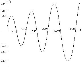
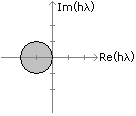
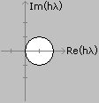
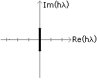
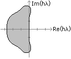
SimplePendulum. Solving equations of motion for a pendulum with frictionless joint.
A simple pendulum whose mass is affected by gravity. No frictional forces
are assumed at the joint. The pairs of images below show the angle of the
pendulum, measured from the vertical, and the region of stability for choosing
the step size of the numerical solver. The Game Physics book goes
into detail about how these pictures are generated.
|
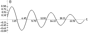
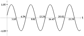
SimplePendulumFriction. Solving equations of motion for a pendulum, friction at joint.
The simple pendulum where the joint has friction. The source code allows
you to overdamp the joint. The pendulum slows down to vertical position with
no oscillation about the vertical. You can also underdamp the problem so
that the oscillations are few (large friction) or so that the oscillations
are many (small friction).
|
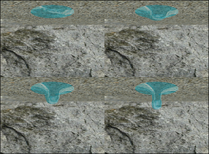
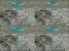
WaterDropFormation. Deformation of revolution surfaces to simulate water-drop formation.
A water drop modeled as a control point surface of revolution. The surface
dynamically changes to show the water drop forming, separating from the main
body of water, then falling to the floor. The evolution is left-to-right,
top-to-bottom.
|
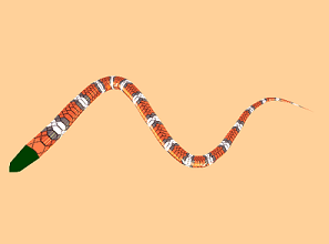
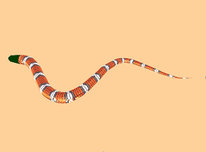
WrigglingSnake. Deformation of tube surfaces to simulate motion of a snake.
Motion of a snake modeled as a tube surface whose central curve is a
control-point medial curve. The curve dynamically changes to simulate
the wriggling.
|