 |
 |
 |
 |
 |
 |
 |
 |
 |
 |
| • | ApproximateBezierCurveByArcs: | Approximate a Bezier curve by circular arcs. |
| • | ApproximateEllipse2: | Least-squares fitting of a set of 2D points by an ellipse. |
| • | ApproximateEllipsesByArcs: | Approximate an axis-aligned ellipse by circular arcs. |
| • | ApproximateEllipsoid3: | Least-squares fitting of a set of 3D points by an ellipsoid. |
| • | BSplineCurveFitter: | Least-squares fitting of points by a B-spline curve. |
| • | BSplineCurveReduction: | Reduction of B-spline curves using a least-squares approach. |
| • | BSplineSurfaceFitter: | Least-squares fitting of points by a B-spline surface. |
| • | FitCone: | Fit a cone to a set of 3D points. |
| • | FitConeByEllipseAndPoints: | Fit a cone to an elliptical cross section and additional points. |
| • | FitCylinder: | Fit a cylinder to a set of 3D points. |
| • | FitTorus: | Fit a torus to a set of 3D points. |
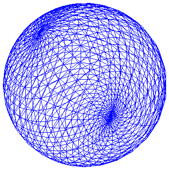
| • | GeodesicEllipsoid: | Compute geodesic paths on an ellipsoid. |
| • | GeodesicHeightField: | Compute geodesic paths on a B-spline-based height-field. |
| • | Interpolation2D: | Various 2D interpolation algorithms. |
| • | NURBSCircle: | Representation of a quarter circle, half circle and full circle using NURBS. |
| • | NURBSCircularArc: | Sample a circular arc represented by one more NURBS curves. |
| • | NURBSCurveExample: | A dynamically varying NURBS curve with topological change. |
| • | NURBSSphere: | Representation of an eighth sphere, half sphere and full sphere using NURBS. |
| • | PartialSums: | GPU-based dynamic programming to compute partial sums of numbers. |
| • | PlaneEstimation: | GPU-based estimation of tangent planes at points in a height field. |
| • | RootFinding: | Root finding of a function of one independent variable; single-threaded, multithread, and on GPU. |
| • | ShortestPath: | Shortest path in a weighted graph (rectangular lattice triangle mesh) (CPU, GPU). |
| • | SymmetricEigensolver3x3: | Special-case iterative eigensolver for a 3x3 symmetric matrix. |
| • | ThinPlateSplines: | Interpolation in 2D and 3D using thin-plate splines. |
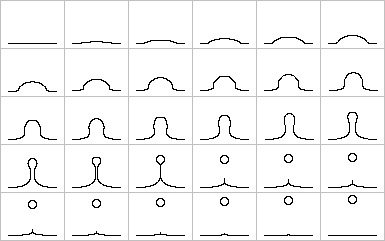
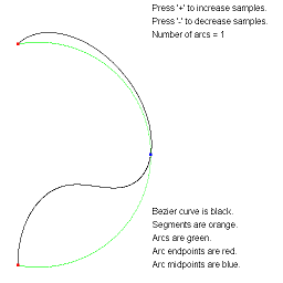
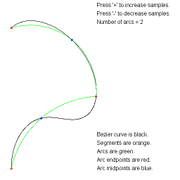
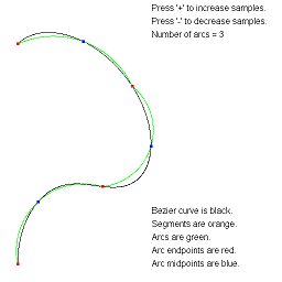
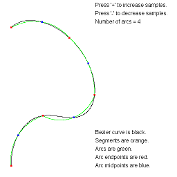
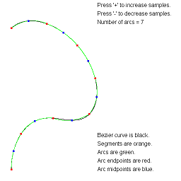
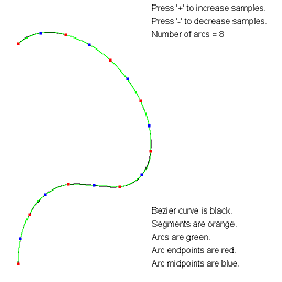
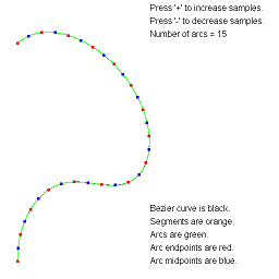
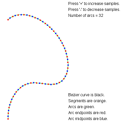
ApproximateBezierCurveByArcs. Approximate a Bezier curve by circular arcs.
The arc-fitting code actually applies to any continuous parametric curve in 2D.
The images show approximations by the specified number of arcs.
The text overlay describes the various objects. You can adjust the
number of arcs using the plus key or minus key.
|
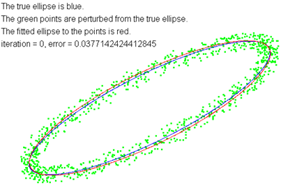
ApproximateEllipse2. Least-squares fitting of a set of 2D points by an ellipse.
The image shows a known ellipse, drawn in blue. The green points are perturbed from
the ellipse by offset points with coordinates in [-1/4,1/4]. The fitted ellipse is
drawn in red.
|
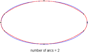
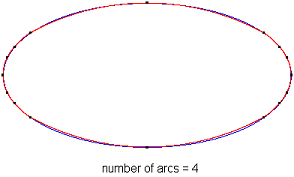
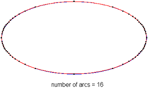
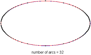
ApproximateEllipseByArcs. Approximate an axis-aligned ellipse by circular arcs.
The images show approximations by the specified number of arcs.
|
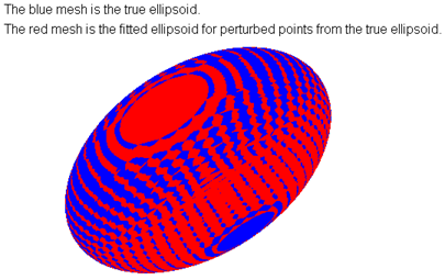
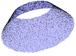
ApproximateEllipsoid3. Least-squares fitting of a set of 3D points by an ellipsoid.
The image shows a known ellipsoid, drawn in blue. Points are perturbed from
the ellipsoid by offset points with coordinates in [-1,1]. The fitted ellipsoid is
drawn in red.
|
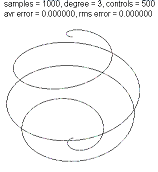
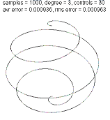
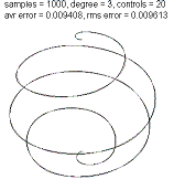
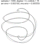
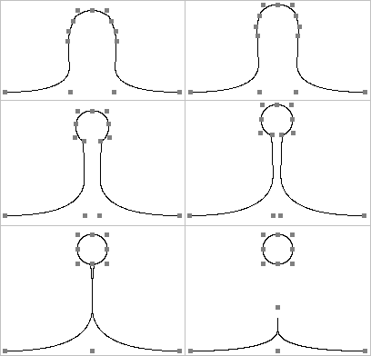
BSplineCurveFitter. Least-squares fit of an ordered sequence of points by a B-spline curve. The
fitting algorithm uses a discrete norm--the sum of squared differences between
the sample points and the corresponding points on the B-spline curve evaluated
at the sample times. The mathematics of this approach is described in the
PDF link and book link but is also described in lesser detail in
The
Essentials of CAGD
by Gerald E. Farin and Dianne Hansford, A. K. Peters,
2000. The approach is common as add-ons to 3D modeling packages for keyframe
compression.
A spiral curve is drawn as a polyline with 1000 vertices. The sample points
are the vertices; think of these as positional keyframes. The sample times
are uniformly spaced. The vertex colors are randomly generated. The fitted
B-spline curves are of degree 3 and drawn as black polylines. Each of the
images shows:
The application keyboard interface allows you to change the degree of the fit using 'D' (increase the degree) or 'd' (decrease the degree). It also allows you to change the number of control points by [small] 's' (decrease by 1) or 'S' (increase by 1), [medium] 'm' (decrease by 10) or 'M' (increase by 10), or [large] 'l' (decrease by 100) or 'L' (increase by 100).
|
BSplineCurveReduction. Reduction of B-spline curves using a least-squares approach. The sample data
points are used as the control points for a B-spline curve. Another B-spline
curve is fitted to the original curve by reducing the number of control
points. The least-squares method is applied to an integral norm, the
integral of the squared distance between the two curves.
The original curve is a sequence of 789 points (from a virtual colonoscopy).
These points are used as the control points for a B-spline curve of degree 3.
The blue curve is the least-squares approximation using an integral norm.
It number of control points is 10 percent of the original points, namely,
78 points. The application allows you to rotate the curves using a virtual
trackball and to move the camera in order to explore the data set.
|
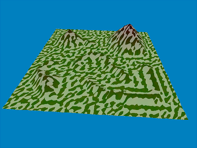
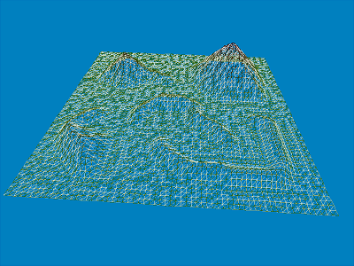
BSplineSurfaceFitter. Least-squares fit of a height field by a B-spline surface. The fitting
algorithm uses a discrete norm--the sum of squared differences between
the sample points and the corresponding points on the B-spline surface
evaluated at the sample parameters. The mathematics of this approach is
described in the PDF link.
The images show a 64x64 height field rendered with a texture containing
shades of green and brown. The height field was fit with a B-spline
surface defined by a 32x32 array of control points. The fitted surface
was resampled to a 64x64 height field for comparison. The fitted surface
has white vertex colors and an alpha channel of one half so that you can
see partially through the surface. The intermixed white patches (fitted)
and green-brown patches (original) make it clear that the fitted surface
stays close to the original, sometimes above it and sometimes below it.
|
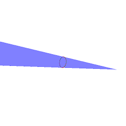
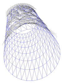
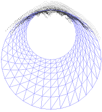
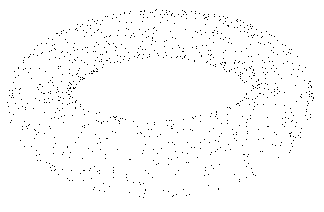
FitCone. Least-squares fit of a cone to a set of 3D points. The mathematics of this approach is
described in the PDF link.
The images show the cone that fits a set of 3D points that are approximately
uniformly distributed on a cone frustum. The left image shows only the
randomly generated sample points. The middle image shows the fitted cone
using Gauss-Newton minimization. The right image shows the fitted cone
using Levenberg-Marquardt minimization. It is difficult to see the difference
but the numerical results are slightly different.
|
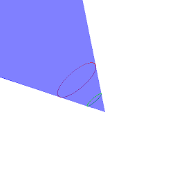
FitConeByEllipseAndPoints. Fit a cone to an elliptical cross section and additional points.
The images show cones that fit elliptical cross sections and some additional
points. The top-left image is a cone that fits a circular cross section and
the cone vertex. The top-right image is a cone that fits a circular cross
section and an elliptical cross section. The bottom-left image shows a cone
that fits two elliptical cross sections. The bottom-right image shows a cone
that fits two partial elliptical cross sections; each ellipse has a portion
truncated by a plane.
|
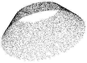
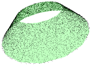
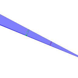
FitCylinder. Least-squares fit of a cylinder to a set of 3D points. The mathematics of this approach is
described in the PDF link.
The images show the cylinder that fits a set of 3D points that are not
uniformly distributed around a cylinder wall. The PDF document has details
and screen captures for other data sets.
|
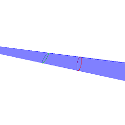
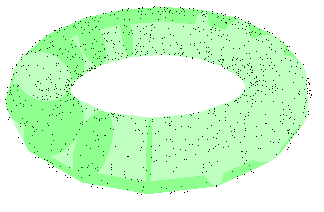
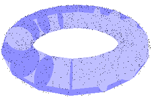
FitTorus. Least-squares fit of a torus to a set of 3D points. The mathematics of this approach is
described in the PDF link.
The images show the torus that fits a set of 3D points that are approximately
uniformly distributed on a torus. The left image shows only the
randomly generated sample points. The middle image shows the fitted torus
using Gauss-Newton minimization. The right image shows the fitted torus
using Levenberg-Marquardt minimization. It is difficult to see the difference
but the numerical results are slightly different. (The changes in coloring are
due to incorrect alpha blending. For simplicity, the points were drawn first
as opaque objects and then the torii are drawn with alpha blending enabled.)
|
GeodesicEllipsoid. Compute geodesic paths on an ellipsoid. The program is set up to compute
geodesic paths on a sphere, something that may be verified analytically. The
sphere may be modified to an ellipsoid in order to compute geodesic paths;
these cannot be verified analytically, because there are no closed-form
equations for these paths.
Two points are randomly generated on a sphere using spherical coordinates.
A point is
(x,y,z) = (cos(theta)*sin(phi),sin(theta)*sin(phi),cos(phi))
In the images here, the points are (theta0,phi0) = (1.116053,0.806658) and
(theta1,phi1) = (0.47751403,0.023537). Pressing the key '0' regenerates a
new pair of points.
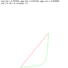
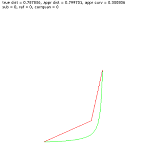
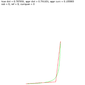
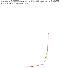
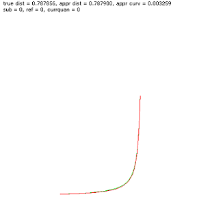
LEFT. The screen represents the (theta,phi) parameter space. The theta variable varies from 0 to pi/2 radians (left to right) and the phi variable varies from 0 to pi/2 radians (top to bottom). The green curve is the geodesic curve in the parameter space. On the sphere, the actual curve is an arc of a great circle connecting the two points. The red line segment is the first approximation (in parameter space) to the geodesic. The error is significant. Notice that the true length is 0.787856 but the approximating curve has length 0.831760. The "appr curv" measurement, 0.893990 in the image, is the integral of the curvature along the approximating curve. Along the geodesic curve, the integral of the curvature is zero since every point on the geodesic has zero curvature. MIDDLE. The application keyboard interface includes key '1' to perform one subdivision of the current polyline and key '2' to perform one refinement for the current subdivision. The next image shows 1 subdivision with 0 refinements. RIGHT. This image shows 1 subdivision with 8 refinements. Notice that the refinements helped move the middle polyline vertex closer to the true geodesic curve. If you were to perform subdivisions only with no refinements at any stage along the way, the approximating curve is not that close to the actual geodesic.
Left: This image shows 1 subdivision, 8 refinements, and 1 more subdivision. Middle: This image shows 1 subdivision, 8 refinements, 1 more subdivision, and then 8 more refinements. Right: This image is a result of 7 subdivisions, each subdivision followed up by 8 refinements. The program takes a long time to run for this configuration. The approximating polyline is close to the actual geodesic. The approximate length is quite close to the true length and the integral of the curvature over the approximating curve is nearly zero.
|
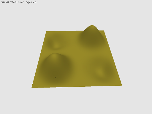
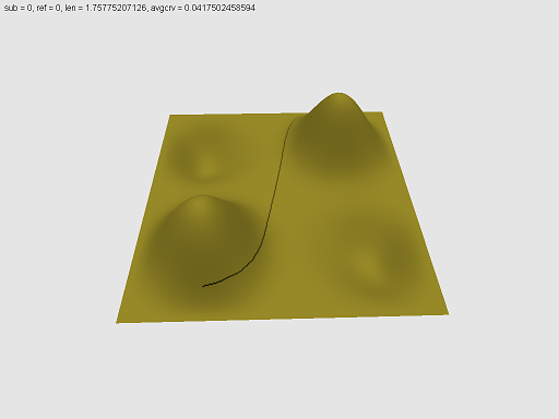
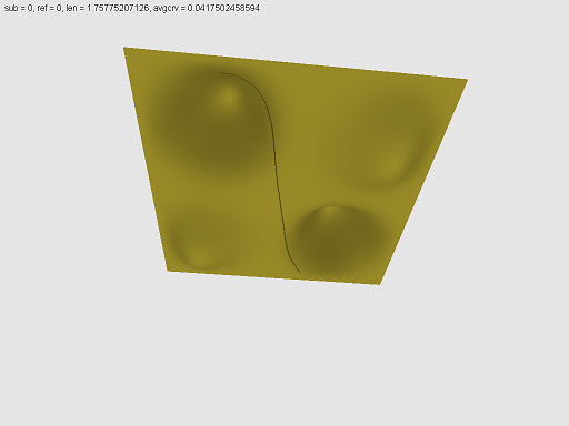
GeodesicHeightField. Compute geodesic paths on a B-spline-based height field
This image shows a B-spline height field, which is defined by the control
points in the file ControlPoints.txt. The surface may be rotated on a
virtual trackball and the camera may be translated using the up- and
down-arrow keys. The small black dot in the image was placed there by a
shift-left-click of the mouse. This point is one endpoint of a geodesic
curve on the height field.
The surface show in the previous image was then rotated so that the first selected point is on the back side of the farthest mountain. A second point was selected on the side of the mountain now facing you. After the selection, the geodesic-path construction occurs. During the construction, you will see the initial geodesic-path approximation evolve and move about the surface. The rendering is somewhat coarse. The curve is plotted on a texture image (of size 512-by-512) and is blended with the lit surface material.
After the construction terminated, the surface was rotated to show you the following bottom-up view. Only 5 subdivisions and 1 refinement per subdivision were used (see the algorithm description in the PDF file). The approximating curve is constructed as a polyline in parametric space. Each line segment in the polyline has a length (in the Riemannian metric, not the straight-line Euclidean length). The total length of the curve approximating the geodesic is shown as 1.85. The integral of the curvature of each line segment in the polyline is computed using a numerical integration. The average of the segment curvatures is shown as 0.15. Ideally, the closer this average is to zero, the better the approximation.
The endpoints in parametric space used in the experiment are
            (u0,v0) = (0.18236097693443298, 0.14066663384437561)
            (u1,v1) = (0.76329755783081055, 0.86457765102386475)
The following list shows the number of subdivisions S, the total length L,
and the average total curvature K.
            S = 5, L = 1.852589, K = 0.158984
            S = 6, L = 1.852097, K = 0.079524
            S = 7, L = 1.852034, K = 0.039778
            S = 8, L = 1.852033, K = 0.019889
As you can see, the larger the number of subdivisions, the smaller the total
length and average total curvature. Visually, there is not much difference
in these curves. Moreover, the computation time grows exponentially with the
increase in subdivisions. The proper balance should be selected for your own
applications.
|
Interpolation2D. An illustration of how to use the various 2D interpolators.
All renderings are in the z-direction, looking down on the height field.
The application allows you to rotate the graph using the virtual trackball
and to toggle wireframe. Both modes allow you to see the differences in
the interpolations.
|
NURBSCircle. NURBS representation of circular components.
A screen capture from the sample application. The
thick green curves are circular components computed using trigonometric
functions. The thin blue curves are the same components computed using
NURBS. The lower left is a quarter circle of degree 2 (Section 2.1.1),
the lower right is a quarter circle of degree 4 (Section 2.1.2), the
upper left is a half circle of degree 3 (Section 2.2) and the upper right
is a full circle of degree 3 (Section 2.3).
|
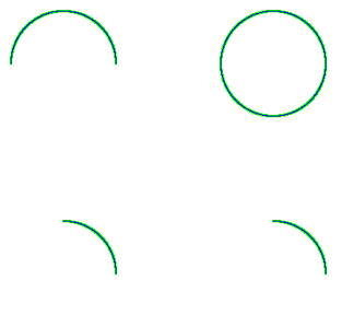
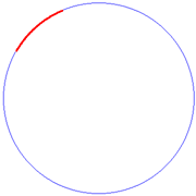
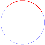
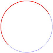
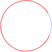
NURBSCircularArc. Sample a circular arc represented by one more NURBS curves.
The blue curves are drawn first and represent the full circle on which the arcs live.
The red curves are drawn as an arc of 3x3 points. The points are computed by the
header file SampleCircularArc.h. The application shows how to draw arcs with various
subtended angles. From left to right, the first image is an arc with angle in 0 to
90 degrees. The second image is an arc with angle in 90 to 180 degrees, but the arc
is a combination of 2 acute arcs. The third image is an arc with angle in 180
degrees to 270 degrees, but the arc is a combination of 3 acute arcs. The fourth
image is an arc with angle in 270 degrees to 360 degrees, but the arc is a
combination of 4 acute arcs.
|
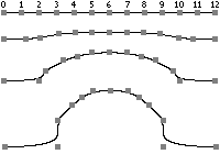
NURBSCurveExample. A dynamically varying NURBS curve with topological change.
Consider a NURBS curve with 13 control points that are initially on the same
straight line. The knot vector is open with uniformly spaced knots. The
curve is necessarily a line segment. The control points must be moved to
deform the central portion of the curve into a closed loop. The control
weights are all 1 except for points 3, 5, 7, and 9, whose weights are 3/10.
These weights were chosen to produce a final closed loop that is nearly
circular. The next image shows the initial line segment and its control
points. It also shows how the control points evolve early in the process.
The next image shows the control points and curves much further along in time. The time sequence is from left to right, then top to bottom. In the lower left image, control points 1 and 11 finally coincide as do control points 2 and 6. At that instant the NURBS curve is split into two NURBS curves as shown in the lower right image. The closed curve has a periodic knot vector. The closed curve continues to move vertically upwards by uniform translations of the control points. The other curve has 5 control points with points 1 and 3 coinciding. The curve evolves back to a line segment by translating the middle control point 2 so that it too coincides with control points 1 and 3.
The next image shows an entire sequence of frames of the deformation. The sequence of images is top row to bottom row, left to right in each row.
|
NURBSSphere. NURBS representation of spherical components.
Screen captures from the sample application. The
left image has an eighth sphere of degree 4 (Section 3.1.2). This is
a triangle-patch surface. The middle image has a half sphere of
degree 3 in each of its 2 parameters (Section 3.2). The right image
has a full sphere of degree 3 in each of its 2 parameters (Section 3.3).
The half and full spheres are rectangular tensor-product patches.
|
| PartialSums. An illustration of a dynamic programming algorithm implemented on a GPU. Partial sums of a sequence of numbers are computed in parallel. If this algorithm were to be implemented sequentially on the CPU, it would be much slower than simply adding the numbers to a running sum. |
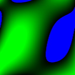
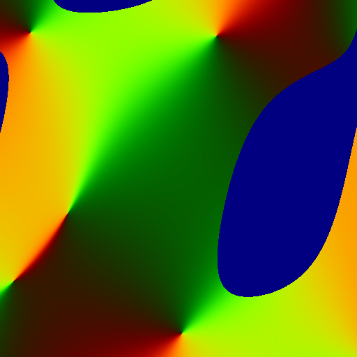
PlaneEstimation. Estimate the tangent plane at every point in a 2D height field using
GPGPU.
The left image shows a bicubic surface in green. The blue regions are "missing data"
(artificially removed). The right image shows a pseudocoloring of the normal
vectors for the estimated tangent planes. No normals are estimated in the regions
of missing data.
|
| RootFinding. Root finding of a function of one independent variable, where computations are performed with 32-bit floating-point arithmetic. These are all exhaustive algorithms, evaluating the function at every finite 32-bit floating-point number. The sequential algorithm on the CPU is slow. A threaded implementation for multiple cores is much faster. The GPU-based algorithm is the fastest. All of these approaches come with a warning: Due to floating-point round-off errors, if a function is expected to have K roots, the algorithms can identify N root bounds where N is larger than K. In this case you need to use a cluster analysis to identify K clusters containing the relevant roots; for example, you could use a K-means clustering algorithm. |
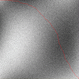
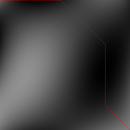
ShortestPath. Compute the shortest path in a weigted graph, which in this sample is
a rectangular array of nodes and each node has three predecessors. The
implementation is GPGPU. A CPU implementation is provided for
comparison, both for performance and to show that the GPU version is not
straightforward--it uses dynamic programming to compute partial sums of
numbers in parallel.
The left image shows a Bezier bicubic gray-scale image with additive random
noise. This image acts as the weights of the graph. The shortest path is
drawn in red. The right image shows the shortest path when no random noise
is added. This path is as you would expect. The path follows dark parts of
the image, initially along the top border. It then steers towards the nearest
saddle point to head towards the dark basin. It then exits the basin and
heads towards the saddle point near the lower-right corner.
|