 |
| • | AdaptiveSkeletonClimbing2: | A multiscale algorithm for segmentation of 2D images. |
| • | AdaptiveSkeletonClimbing3: | A multiscale algorithm for segmentation of 3D images. |
| • | BSplineInterpolation: | Illustrates how to use B-spline interpolation on any dimension image. |
| • | Convolution: | Various algorithms for convolution of an image with a separable kernel (GPU). |
| • | ExtractLevelCurves: | Extract level curves from a 2D gray-scale image. |
| • | ExtractLevelSurfaces: | Extract level surfaces from a 3D gray-scale image. |
| • | ExtractRidges: | Extract 1D ridges and valleys from a 2D image. |
| • | GaussianBlurring: | GPU-based image convolution using ping-pong buffers. |
| • | GpuGaussianBlur2: | Gaussian blurring of a 2D image, implemented using a GPU. |
| • | GpuGaussianBlur3: | Gaussian blurring of a 3D image, implemented using a GPU. |
| • | MedianFiltering: | Fast median filtering using 3x3 or 5x5 windows (GPU). |
| • | SurfaceExtraction: | Extraction of level surfaces from 3D images (GPU). |
| • | VideoStreams: | A producer-consumer model to upload images to the GPU while processing the images in parallel. |
| AdaptiveSkeletonClimbing2. A multiscale algorithm for segmentation of 2D images. The sample program is very basic, enough to verify that the code is working. |
| AdaptiveSkeletonClimbing3. A multiscale algorithm for segmentation of 3D images. The sample program is very basic, enough to verify that the code is working. |
| BSplineInterpolation. Illustration of B-spline interpolation for 1D, 2D and 3D images. The B-spline interpolation class supports any dimension (even larger than 3) and allows for compile-time-specified dimension or run-time-specified dimension. The 1D example is from the B-spline interpolation PDF, the end of example 1 near the bottom of page 7. The 2D example is a resampling of a 2D color image. The 3D example is a resampling of a 3D x-ray crystallography image. |
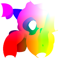
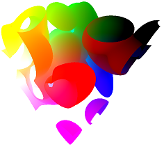
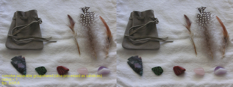
Convolution. Various GPU-based algorithms for convolution of an image with a
separable kernel are illustrated. Direct convolution applies
the kernel as a 2D entity. Separability is used to show how much
faster it is to use horizontal and vertical passes. The examples
also include using group-shared memory in the compute shaders.
The interface allows you to toggle through various modes: convolve as a 2D kernel,
convolve as a 2D kernel using group-shared memory, convolve by a 1D horizontal
kernel followed by a 1D vertical kernel, convolve with 1D kernels but using
group-shared memory, and the image is partitioned into subimages and each subimage
is convolved with 1D kernels using group-shared memory. The image here shows the
last case.
|
|
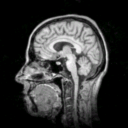
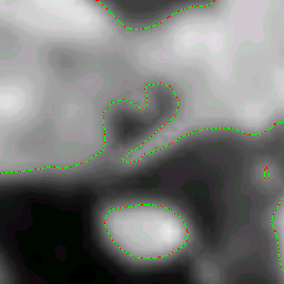
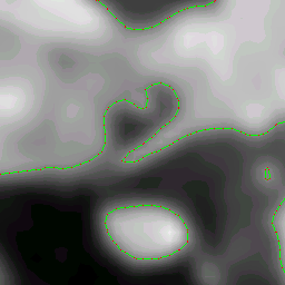
ExtractLevelCurves. Extract level curves from a 2D gray-scale image.
Left: The original image is a gray scale MRI slice of size 256-by-256 (the
"Chapel Hill Head").
Middle and right: These images are zoomed copies of the 32-by-32 subimage with origin at (100,100) in the original image. The left image used extraction by decomposing each square pixel into two triangles and assuming a linear interpolation on each triangle. The right image used extraction by assuming a bilinear interpolation on each square pixel.
|
ExtractLevelSurfaces. Extract level curves from a 3D gray-scale image.
CUBE EXTRACTION.
Each voxel has eight corners that are data samples. The image values within
the voxel are assumed to be generated by trilinear interpolation. That means
the faces are bilinearly interpolated and the edges are linearly
interpolated. The extraction was applied using level value 64 in the
superoxide dismutase molecule image (molecule.im).
The method implemented here is not the Marching Cubes Algorithm (MCA). The MCA assumes linear interpolation of edges to find intersections of the level surface with the voxel. As long as the level set value is a non-image value, the level surface can only intersect interior edge points. As a result, there are 256 possible intersection configurations with the edges based on whether the differences between the image values at the voxel corners and the level set value are positive (sign +1) or negative (sign -1). The MCA has a precomputed table of 256 different triangle meshes whose lookup value is determined by the signs at the voxel corners. This can lead to topological problems on a face shared by two voxels. The PDF documentation file explains how the topological problem arises and shows how it is avoided. Moreover, the extraction algorithm provided here is topologically correct in the sense that the triangle mesh has the same number of connected components and same topology as the true level surface of the trilinear function. The triangle mesh in a voxel is not obtained as a table lookup. It is constructed by a simple ear-clipping algorithm applied to the wireframe edges constructed on the faces of the voxel. TETRAHEDRON EXTRACTION. Each voxel is decomposed into five tetrahedra and linear interpolation is assumed on each tetrahedron. The extraction was applied using level value 64 in the superoxide dismutase molecule image (molecule.im). The left image is a view from outside the entire voxel data set. The right image is a view where the camera is moved closer to the data set. Back-face culling is disabled to make sure that non-closed surfaces are viewable from any orientation. The polygonal models have a single material and the scene is illuminated with two directional lights. Notice that the large component in the lower right of the right image is an open surface. This component has its boundary curve on a plane of the voxel data boundary (effectively a truncated portion of a closed surface).
|
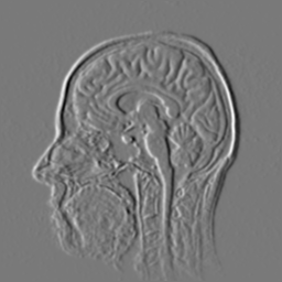
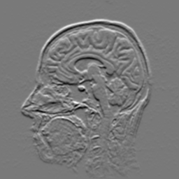
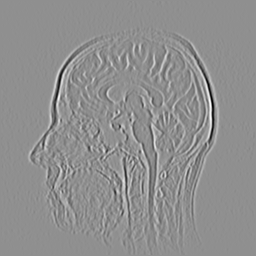
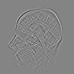
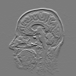
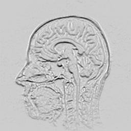
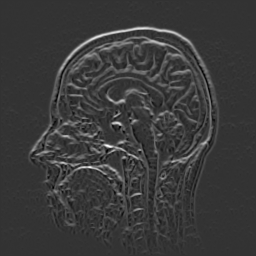
ExtractRidges. Extract 1D ridges and valleys from a 2D image. The segmentation in this sample is crude
in the sense that only the pixels are classified without any attempt to
coalesce them into curves. The goal of the sample is to illustrate the
mathematical concepts.
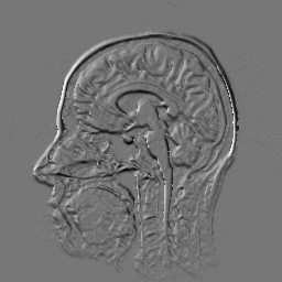
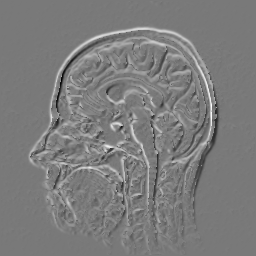
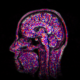
The first-row-left image is the original image (slice from a 3D MRI). The
first-row-middle image is the x-derivative (using finite differences). The
first-row-right image is the y-derivative. The second-row-left image is the
second-order xx-derivative. The second-row-middle image is the xy-derivative.
The second-row-right image is the yy-derivative. Let H be the symmetric
matrix of second-order derivatives The third-row-left image is the minimum
eigenvalue of H. The third-row-middle image is the maximum eigenvalue of H.
The third-row-right image is the derivative in the direction of the eigenvector
corresponding to the minimum eigenvalue. The fourth-row-left image is the
derivative in the direction of the eigenvector corresponding to the maximum
eigenvalue. The fourth-row-middle image is the classification. Ridge points
occur when the minimum eigenvalue is negative and the corresponding directional
derivative is zero (showin in red). Valley points occur when the maximum
eigenvalue is positive and the corresponding directional derivative is zero
(shown in blue). Saddle points are those classified both as ridge and valley
points (shown in magenta).
|
GaussianBlurring. Gaussian blurring using a 3x3 kernel and ping-pong buffers.
The left image is the original. The middle image is the output of 100 passes
of Gaussian blurring. The right image is the output of 1000 passes of Gaussian
blurring. The shader does not do special processing on the image boundary pixels,
so the shader performs out-of-range lookups for pixels outside the image. HLSL
specifications require the lookups to be zero-valued, which is why the black band
around the boundary occurs.
|
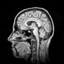
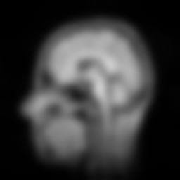
GpuGaussianBlur2. Gaussian blurring of a 2D image, implemented using a GPU.
The left image is the original image (256x256 slice of an MRI). The right
image is a blurred copy after a moderate number of iterations of the numerical
solver.
|
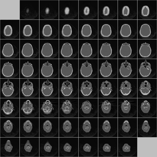
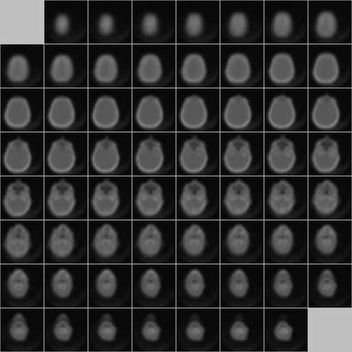
GpuGaussianBlur3. Gaussian blurring of a 3D image, implemented using a GPU.
The left image is the original 3D image (128x128x64 CT scan) drawn as a tiled
2D image. The right image is a blurred copy after a moderate number of
iterations of the numerical solver.
|
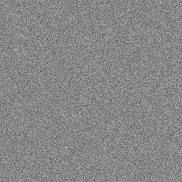
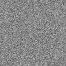
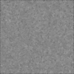
MedianFiltering. GPU-based median filtering using 3x3 or 5x5 windows. The algorithm uses
swapping of channels of 4-tuples using minimum and maximum operators,
which is much faster than an insertion sort performed in the compute
shader.
The left (input) image is randomly generated. The middle image is the output
from 3x3 median filtering. The right image is the output from 5x5 median
filtering. The images themselves are not important. The goal is to show
how fast median filtering can be on the GPU.
|
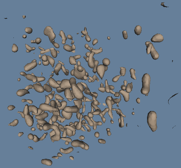
SurfaceExtraction. GPU-based extraction of level surfaces from a 3D voxel data set. The
algorithm uses a Marching-Cubes-like table lookup for constructing the
triangles contained in a voxel that the surface intersects. The example
uses extraction and display using a standard vertex shader that takes
as input elements from a vertex buffer. For comparison, a vertex shader
is implemented that uses the SV_VERTEXID semantic for passing indices
into a buffer that represents the vertices. This approach is much
faster, because the output of the compute shader that performs the
surface extraction cannot be a vertex buffer resource. The standard
vertex shader requires that an extra round-trip memory copy between
GPU and CPU, which you want to avoid.
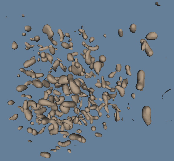
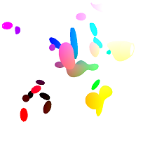
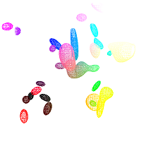
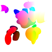
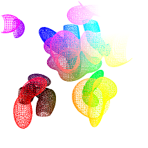
The 3D image is create as a sum of 32 Gaussian distributions whose means
and covariance matrices are randomly generated. The image is then scaled
to have values in the interval [0,1]. The first two images show the surfaces
extracted for level value 0.5. The second two images show the surfaces for level
value 0.15. The last two images show the surfaces for level value 0.01 for two
different orientations of the virtual trackball.
|
| VideoStreams. The video-stream sample shows how you can upload images to the GPU using a producer-consumer model. The upload and subsequent resource creation is in a thread different from the main thread where the image processing is initiated on the GPU. This is a useful pattern to use to parallelize resource creation and computing with those resources. |