|
 |
 |
 |
 |
 |
 |
 |
 |
 |
 |
 |
 |
 |
| • | CLODPolyline: | Continuous level of detail for a polyline (decimation by vertex collapses). |
| • | ConformalMapping: | Conformal mapping of a triangle mesh of genus 0 onto a sphere. |
| • | ConstrainedDelaunay2D: | Constrained Delaunay triangulation that uses exact rational arithmetic (CPU). |
| • | ConvexHull2D: | Convex hull for a set of 2D points that uses exact rational arithmetic (CPU). |
| • | ConvexHull3D: | Convex hull for a set of 3D points that uses exact rational arithmetic (CPU). |
| • | ConvexHullSimplePolygon: | Convex hull for a simple polygon with vertices in counterclockwise order. |
| • | Delaunay2D: | Delaunay triangulation for a set of 2D points that uses exact rational arithmetic (CPU). |
| • | Delaunay3D: | Delaunay tetrahedralization for a set of 3D points that uses exact rational arithmetic (CPU). |
| • | DisjointIntervalsRectangles: | Boolean operations on intervals and axis-aligned rectangles. |
| • | ExtremalQuery: | Compute extreme points for convex polyhedron using BSP trees. |
| • | GenerateMeshUVs: | Automatic generation of texture coordinates for a mesh with rectangle or disk topology. |
| • | IncrementalDelaunay2: | Incremental insertion/removal of points for Delaunay triangulation. |
| • | MinimalCycleBasis: | Extract all the cycles from a planar graph as a forest of cycle-basis trees. |
| • | MinimumAreaBox2D: | Minimum-area or minimum-width bounding box for a set of 2D points that uses exact rational arithmetic (CPU). |
| • | MinimumAreaCircle2D: | Minimum-area circle for a set of 2D points that uses exact rational arithmetic (CPU). |
| • | MinimumVolumeBox3D: | Minimum-volume bounding box for a set of 3D points that uses some exact rational arithmetic (CPU). |
| • | MinimumVolumeSphere3D: | Minimum-volume sphere for a set of 3D points that uses exact rational arithmetic (CPU). |
| • | PolygonBooleanOperations: | Boolean operations on polygons (union, intersection, difference, exclusive-or) using BSP trees. |
| • | SplitMeshByPlane: | A simple algorithm for clipping a triangle mesh by a plane. |
| • | TriangulationEC: | Triangulation via ear clipping of polygons, nested polygons, and trees of nested polygons. |
| • | TriangulationCDT: | Triangulation via constrained Delaunay triangulation of polygons, nested polygons, and trees of nested polygons. |
| • | VertexCollapseMesh: | Vertex collapses to decimate a mesh while preserving the mesh topology. |
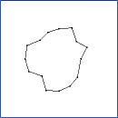
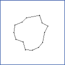
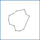
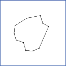
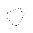
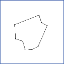
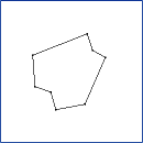
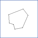
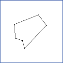
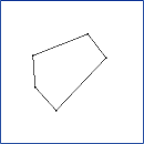
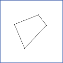
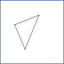
CLODPolyline. Continuous level of detail for a polyline
(decimation by vertex collapses). Each vertex V[i] is some distance
to the line segment connecting its neighbors, V[i-1] and V[i+1]. To
reduce the level of detail, the vertex of minimum distance is removed
from the polyline. This example illustrates the min-heap data
structure designed for geometric algorithms.
The sequence of images is ordered from top row to bottom row. Within each row, the
ordering is from left column to right column. The application keyboard interface
allows you to adjust the level of detail: '+' to increase the level of detail or
'-' to decrease the level of detail.
|
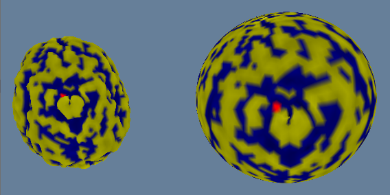
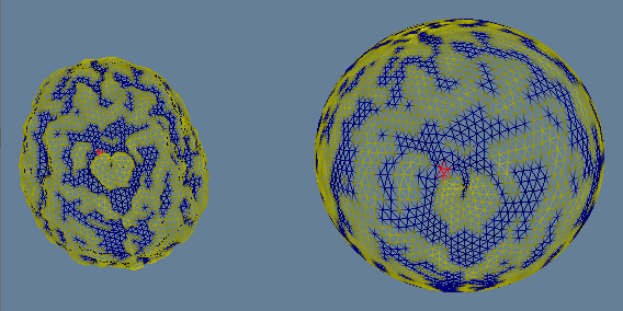
ConformalMapping. Conformal mapping of a triangle mesh of genus
0 onto a sphere while minimizing distortion. The method is useful for
generating texture coordinates on the original triangle mesh. The
spherical coordinates act as the texture coordinates.
The images show the original mesh on the left (a brain surface segmented from
a 3D medical image) and the conformally mapped sphere on the right. The
vertices are pseudocolored according to mean curvature. The vertices of the
puncture triangle are set to red, so that triangle shows up as red;
neighboring triangles get interpolated values based on the red vertex and
their other pseudocolored vertices. You can see that the conformally mapped
mesh has a minimum of distortion compared to the original.
|
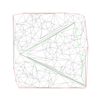
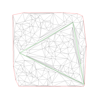
ConstrainedDelaunay2D. Constrained Delaunay triangulation. This is a CPU implementation that
uses exact rational arithmetic for a robust (and correct) algorithm.
The unsigned integer type for the exact arithmetic uses a fixed-size
structure for speed. Of course, you need to determine how many bits of
precision are required for your algorithm in order to use a fixed-size
structure.
The row0-column0 image shows the Delaunay triangulation of a random set
of points. The green edges are required to be part of the triangulation.
The row0-column1 image shows the triangulation after inserting one green
edge. The row1-column0 image shows the triangulation after insertion another
green edge. Thw row1-column1 image shows the triangulation after insertion
of the final green edge.
|
ConvexHull2D. Convex hull of 2D points. This is a CPU implementation that uses exact
rational arithmetic for a robust (and correct) algorithm. The unsigned
integer type for the exact arithmetic uses a variable-size structure, so
a large portion of the execution time is spent allocating and
deallocating memory. Feel free to determine how many bits of precision
are required and switch to a fixed-size structure instead in order to
improve the performance.
The left image shows the convex hull of a random set of 2D points. The
right image shows the convex hull of a 3x3 grid of points. The 3x3 grid
is a typical data set that causes problems when using floating-point
arithmetic, because the set has collinear points and the classification
of collinearity using signs of determinants might be incorrect due to
round-off errors.
|
ConvexHull3D. Convex hull of 3D points. This is a CPU implementation that uses exact
rational arithmetic for a robust (and correct) algorithm. The unsigned
integer type for the exact arithmetic uses a fixed-size structure for
speed. Of course, you need to determine how many bits of precision are
required for your algorithm in order to use a fixed-size structure.
The images show the convex hull of various data sets. These data sets
(courtesy of John Ratcliff) were ones that failed the floating-point-only
algorithm in an earlier version of Wild Magic (leading to some scrambling
to make that algorithm more robust). All hulls are computed correctly with
the exact arithmetic of GTEngine.
|
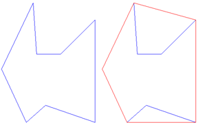
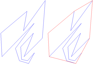
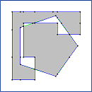
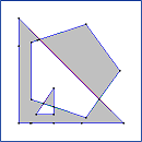
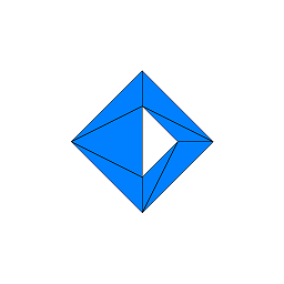
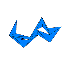
ConvexHullSimplePolygon. Convex hull of a simple polygon with vertices in
counterclockwise order.
The code can be executed either with floating-point arithmetic or rational
arithmetic. The left image shows the convex hull (drawn in red) of a
geometrically simple polygon (drawn in blue). The right image shows the
convex hull of a geometrically complicated polygon (using blue and red as
for the left image). The header file for the implementation has other links
of interest for the algorithm.
|
|
Delaunay2D. Delaunay triangulation. This is a CPU implementation that uses
exact rational arithmetic for a robust (and correct) algorithm. The
unsigned integer type for the exact arithmetic uses a variable-size
structure, so a large portion of the execution time is spent allocating
and deallocating memory. Feel free to determine how many bits of
precision are required and switch to a fixed-size structure instead in
order to improve the performance.
The left image shows the Delaunay triangulation of a random set of 2D points.
The middle image shows the linear-walk search algorithm for locating a triangle that contains a point. The green triangle is where the user clicked the left-mouse button. An initial triangle is selected and the binary-space partitioning tree implied by the triangulation is used to guide the search path to that triangle. The initial triangle is on the boundary of the triangulation, and the path leads vertically upward. You can save the last containing triangle and specify that as the starting triangle for the next search query. For spatially coherent point selections, such as in resampling of meshes for interpolation, this provides effectively an O(1) algorithm for searching. The right image shows the Delaunay triangulation for a 3x3 grid of points. This is a typical data set that cause problems for floating-point implementations because of the presence of cocircular points.
|
|
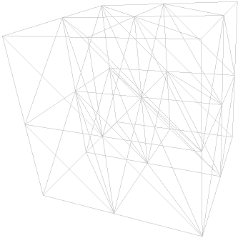
Delaunay3D. Delaunay tetrahedralization. This is a CPU implementation that
uses exact rational arithmetic for a robust (and correct) algorithm.
The unsigned integer type for the exact arithmetic uses a fixed-size
structure for speed. Of course, you need to determine how many bits
of precision are required for your algorithm in order to use a
fixed-size structure.
The left image shows the Delaunay tetrahedralization of a set of random 3D points.
The middle image shows a linear walk, similar to that in 2D, to find a tetrahedron containing a query point. In this example, the query point is shown as a small black sphere. The search path starts with a purple-colored tetrahedron. The final tetrahedron is colored red. The tetrahedra from start to finish have increasing red channel and decreasing blue channel. In practice, the linear walk is an efficient algorithm, but it is known that there exist (pathological) data sets for which the search algorithm is quadratic in time. The right image shows the Delaunay tetrahedralization of a 3x3x3 grid of points. This is a typical data set that cause problems for floating-point implementations because of the presence of cospherical points.
|
| DisjointIntervalsRectangles. Boolean operations on intervals and on axis-aligned rectangles (union, intersection, difference, exclusive-or). The application has no visual output and act as unit tests for the engine code. |
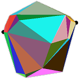
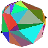
ExtremalQuery. Compute extreme points for convex polyhedron using BSP trees.
The application displays a convex polyhedron, each face having a distinct color.
The extreme points in the x-direction (left/right) are shown as small black
spheres. The polyhedron is on a virtual trackball. As you rotate it with a
left-drag of the mouse, the extreme points change dynamically. The left image
shows the initial configuration of the polyhedron. The right image shows the
polyhedron slightly rotated from top to bottom.
|
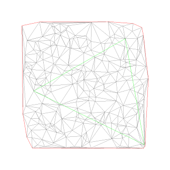
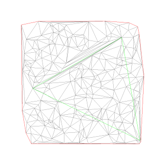
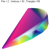
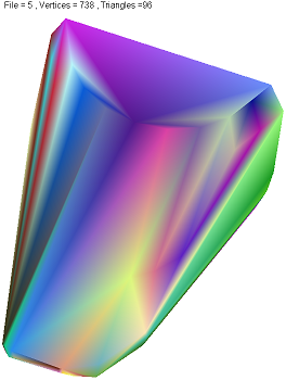
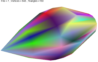
GenerateMeshUVs. Automatic generation of texture coordinates for a mesh with rectangle or disk topology.
The first pair of images (from left to right) show the original mesh, which was generated
from a hemisphere using random perturbations of the spherical points along rays.
The texture coordinates were generated manually (using the MeshFactory class).
The second pair of images show a mesh whose texture coordinates were generated
by the class GenerateMeshUV; the comments in the class header list the reference
for the algorithm. The mesh was then resampled in uv-space. The left images
of the pairs are renderings of the meshes and the right images of the pairs are
corresponding wireframe renderings of the meshes so that you can see the underlying
uv-mesh. The orientations of the texture on the two meshes are different, because the
orientation using barycentric mapping dependns on how the mesh boundary is
mapped to the boundary of the uv-square.
|
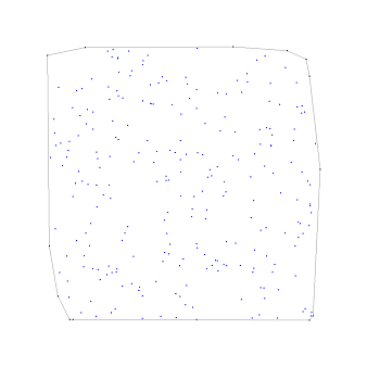
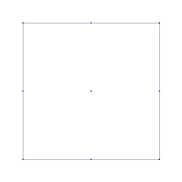
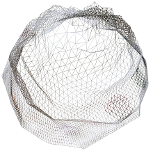
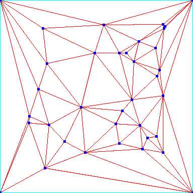
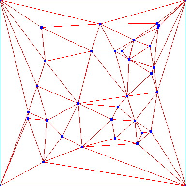
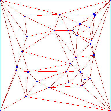
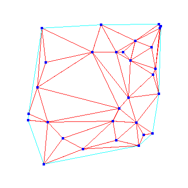
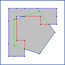
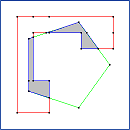
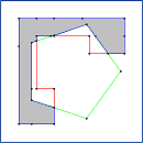
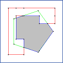
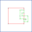
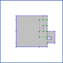
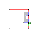
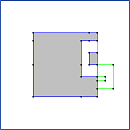
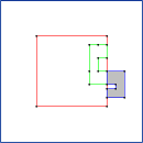
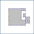
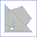
IncrementalDelaunay2. Incremental insertion and removal of points for a Delaunay
triangulation. The code uses a blend of interval arithmetic and rational arithmetic to
ensure correct results.
The constructor of IncrementalDelaunay2 requires you to specify a bounding rectangle
for the points you plan on inserting or removing. A supertriangle is created to contain
the bounding rectangle. The rectangle itself is inserted into the triangulation (as 2
triangles). The upper-left image is the initial triangulation of 32 points, inserted with
32 insert operations. The triangles are drawn in red and the convex hull is drawn in blue.
The hull is the bounding rectangle. The upper-right image has the lower-right-most point
removed (via a SHIFT plus LEFT-MOUSE-DOWN operation). The lower-left image is the
upper-right image with an interior point removed--the point approximately left of center
in the upper-right image. When you are finished with insertions and removal of points,
you can keep the bounding rectangle if your application requires it. If you do not want
the bounding rectangle, a member function FinalizeTriangulation() can be called to remove
it. Once called, you can no longer insert or remove points; that is, the triangulation is
final. The lower-right image is obtained by calling FinalizeTriangulation() for the
lower-left image. The convex hull edges are drawn in cyan; these edges are part of the
Delaunay triangulation.
|
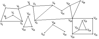
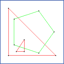
MinimalCycleBasis. Extract all the cycles from a planar graph as a forest of cycle-basis trees.
The algorithm is described in the PDF document.
The SimpleGraph1.txt file contains the information for a graph of 26 vertices
and 30 edges. The left image shows the graph with labeled vertices. The
right image shows the extracted forest of cycle-basis trees.
|
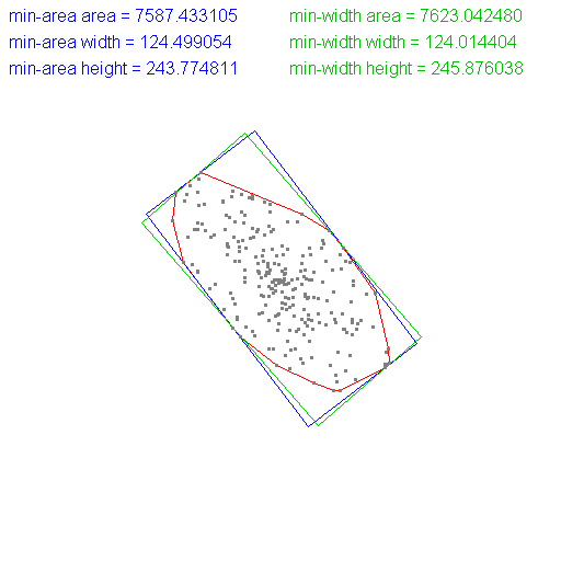
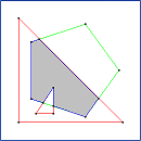
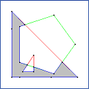
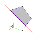
Minimum-area or minimum-width box containing a set of 2D points. These are CPU
implementations that use exact rational arithmetic for a robust (and
correct) algorithm. The minimum-area box requires you to specify the rational
compute type. This will change with when GTL ships because the class will handle
the exact arithmetic and precision internally. The minimum-width box already
hides the exact arithmetic.
The minimum-area box containing a set of 2D points randomly generated within
an oriented ellipse is shown in the image. The convex hull of the points
is drawn in red. The minimum-area box is drawn in blue. The minimum-width box
is drawn in green. Observe that the two boxes are not the same.
|
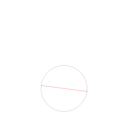
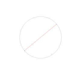
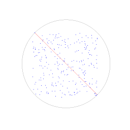
MinimumAreaCircle2D. Minimum-area circle containing a set of 2D points. This is a CPU
implementation that uses exact rational arithmetic for a robust (and
correct) algorithm. The unsigned integer type for the exact arithmetic
uses a variable-size structure, so a large portion of the execution time
is spent allocating and deallocating memory. Feel free to determine how
many bits of precision are required and switch to a fixed-size structure
instead in order to improve the performance.
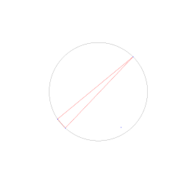
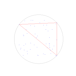
The sample displays the minimum-area circle as you insert each point one
at a time. The first row of images (left to right) show insertion of two,
three, and four points. The next row, first column. shows insertion of many but not
all of the points. The last image shows insertion of all the point; in this
example, the minimum-area circle is supported by two points.
|
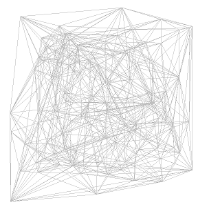
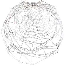
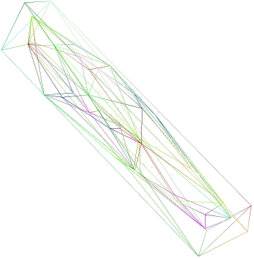
MinimumVolumeBox3D. Minimum-volume box containing a set of 3D points. This is a CPU
implementation that uses exact rational arithmetic to compute the convex
hull of the points. The minimum-volume box is selected from those boxes
that are coincident with a face of the hull or with three perpendicular
edges of the hull. The algorithm requires projection onto planes and
lines, and it is not tractible to compute with exact rational arithmetic.
This portion of the algorithm switches to floating-point arithmetic, so
there is the potential for round-off errors that leads to a box that is
close to, but not, the theoretical minimum-volume box.
The minimum-area box containing a set of 3D points randomly generated within
an oriented ellipsoid is shown in the image. The wireframe of the convex hull
of the points is visible as well as the wireframe of the bounding box.
|
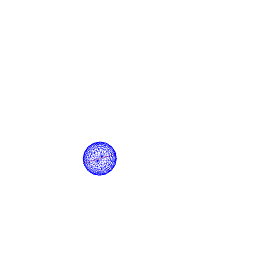
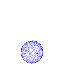
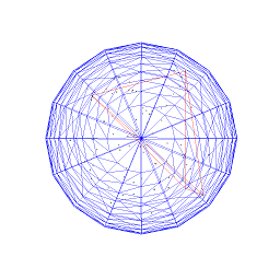
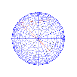
MinimumVolumeSphere3D. Minimum-volume sphere containing a set of 3D points. This is a CPU
implementation that uses exact rational arithmetic for a robust (and
correct) algorithm. The unsigned integer type for the exact arithmetic
uses a variable-size structure, so a large portion of the execution time
is spent allocating and deallocating memory. Feel free to determine how
many bits of precision are required and switch to a fixed-size structure
instead in order to improve the performance.
The sample displays the minimum-volume sphere as you insert each point one
at a time. The first row of images (left to right) show insertion of two,
three, and four points. The next row, first column. shows insertion of many but not
all of the points. The last image shows insertion of all the point; in this
example, the minimum-volume sphere is supported by four points.
|
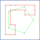
PolygonBooleanOperations. Boolean operations on polygons (union, intersection, difference,
exclusive-or). The implementation uses binary space partitioning (BSP)
trees. Although easy to implement, it generates too many small line
segments when you have a lot of polygons in the system. A better
approach is to use a sort-and-sweep algorithm for computing
edge-edge intersections.
The following images show the application of the algorithm to three different
pairs of polygons. The black dots indicate all the points generated by the
BSP tree construction. There are many more points than are necessary to
actually compute the Boolean results. After applying Boolean operations, you
may eliminate some of these points by checking for triples of collinear
points.
|
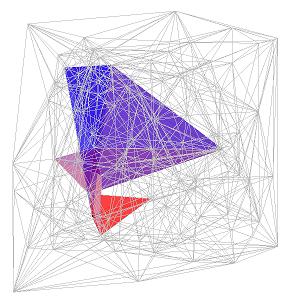
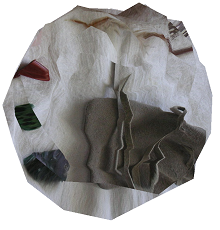
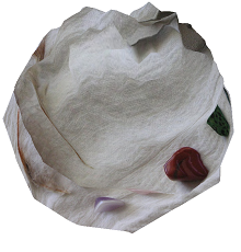
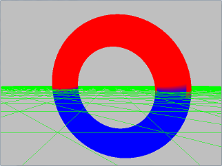
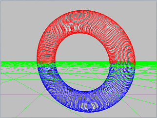
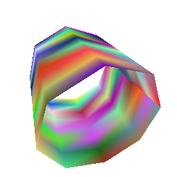
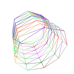
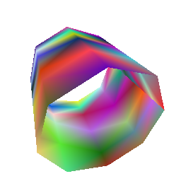
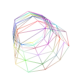
SplitMeshByPlane. A simple algorithm for clipping a triangle mesh by a plane.
The two images show the mesh clipped by the plane. Triangles above the plane
have vertices drawn in red. Triangles below the plane have vertices drawn in
blue. Vertices that are part of both meshes are drawn in purple. You can
rotate the torus in real time, seeing the meshes change over time.
|
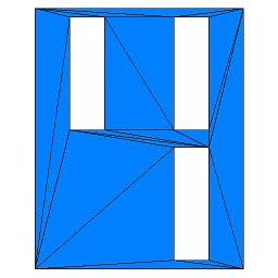
TriangulationEC. Triangulation via ear clipping of polygons, nested polygons, and trees of nested polygons.
In the first row, the triangulation of a simple polygon is shown in the
left image. The middle image shows a polygon with a single hole. The right
image shows a polygon with two holes. In the bottom row, the left image is
the triangulation of a tree of nested polygons. The right image is the
triangulation of a polygon with three holes. The sample code generates the
triangulations for each of the six possible orderings of the holes, leading
to valid triangulations in all cases.
|
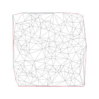
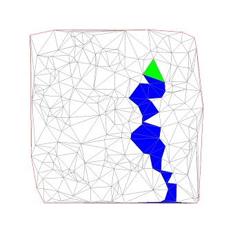
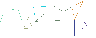
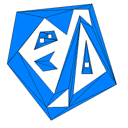
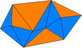
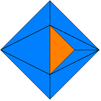
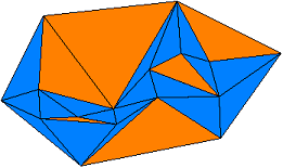
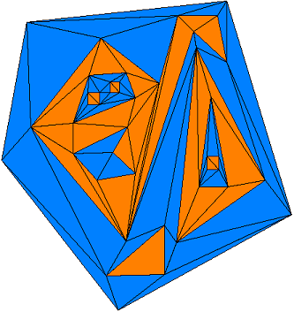
TriangulationCDT. Triangulation via constrained Delaunay triangulation of polygons, nested polygons, and trees of nested polygons.
The TriangulateCDT class produces a convex hull of the polygon vertices and requires
that the polygon edges are in the triangulation. The triangles are either inside or outside
the polygon. Those inside form the triangulation of the polygon. However, having the convex hull is
useful for applications that want to test for triangle containment. You can use a PlanarMesh
object of the output triangles, which allows you to determine which triangle contains the query
point. That triangle's index can be passed to a TriangulateCDT function that tells you
whether the triangle is inside or outside the triangulation. A typical application might be
interpolation of function data that is defined on a nonconvex domain.
The sample application uses the same polygons as for TriangulationEC. However,
a PlanarMesh object is built from the triangulation. Each pixel in the
image is sent to a point-in-triangle query. If in a triangle, a query is made
to determine whether it is inside or outside the polygon triangulation. If inside,
the pixel is colored blue; if outside, the pixel is colored orange.
|
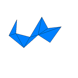
VertexCollapseMesh. Vertex collapses to decimate a mesh while preserving the mesh topology.
The top row of images is the original mesh, an approximation to a cylinder, and is
shown as a solid surface and as a wireframe surface. The bottom row of images is
the mesh with 12 vertex collapses applied.
|